Statistics Case Studies: Movies and Stock Market Prices
The purpose of this document is to use descriptive and inferential statistics to draw conclusions about data sets, e.g. a data set about 100 movies, containing opening gross, total gross, number of theaters, and weeks in the top 60, as well as a data set concerning stock prices over time for eight companies.
Movies
Descriptive Statistics
| Statistic | Opening Gross | Total Gross | Number of Theaters | Weeks in Top 60 |
| Mean | $9.37 | $33.04 | 1278 | 8.68 |
| Median | $0.39 | $5.85 | 410 | 7 |
| Mode | $0.03 | NA | 202 | 1 |
| Standard Deviation | $18.87 | $63.16 | 1379 | 6.4 |
| High | $108.44 | $380.18 | 3910 | 27 |
| Low | $0.01 | $0.03 | 5 | 1 |
| Skew | 3.43 | 3.28 | 0.56 | 0.67 |
| Range | $108.43 | $380.15 | 3905 | 26 |
Table 1. Descriptive Statistics for 100 movies
Descriptive statistics were calculated for the movies data set using Microsoft Excel (Table 1). There was a wide variation in the performance of the 100 movies, but the median Total Gross of $5.85, as compared to the mean of $33.04, suggests that only a few movies performed exceptionally well. The mean opening gross was $9.37 M, with a standard deviation of $18.87. It should be noted that the standard deviation is twice the value of the mean! This is due to the large skew (3.43) in the data, which, since it is positive, indicates a long tail towards the right. Comparing the high value with the mean ($108.44 versus $9.37) also suggests that the data is extremely skewed. The range was $108.43 M, with high of $108.44 and low of $0.01.
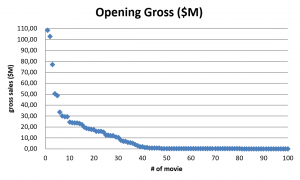
Figure 1. Opening Gross ($M)
As can be seen in the graph (Figure 1), there are five main high-performing outliers (Star Wars: Episode III, Harry Potter and the Goblet of Fire, War of the Worlds, Mr. and Mrs. Smith, and Batman Begins), with gross sales between $40 M and $110 M. The skewness of the data is also evident with the extremely long tail to the right (notes that the data points were rank ordered before the graph was created).
The mean total gross was $33.04 M, the median was $5.85 M, and the mode was unavailable because several numbers appeared twice but none more than twice. The standard deviation, like that of the opening gross, was approximately twice the mean at $63.16 M. Not surprisingly, the skew was 3.28. The high point was $380.18 M and the low point was $0.03 M, with a range of $380.15 M.
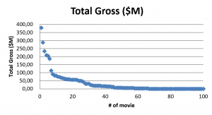
Figure 2. Total Gross Sales ($M)
In the graph (Figure 2) of the total gross sales, seven outliers can be seen between $100 M and $400 M. Also evident is the positive skew mentioned earlier.
The mean of the number of theaters was 1278, with a median of 410, and mode of 202. The standard deviation of 1379, was somewhat greater than the mean, which suggests a positive skew, but not a large one; skew was calculated to be 0.56. The high value was 3910, and low was 5. The range was 3905. The graph (Figure 3) did not show outliers as in the first two.
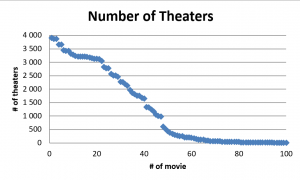
Figure 3. Number of Theaters.
The mean of the weeks each movie spent in the top 60 was 8.68, with a median of 7, and mode 1. The standard deviation was 6.4, lower than the mean; skew was calculated to be 0.67. The high value was 27, and low was 1. The range was 26. The graph (Figure 4) showed 1 outlier of 27.
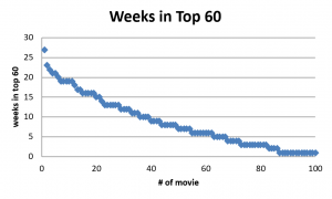
Figure 4. Weeks in Top 60.
Correlations
Correlations were computed to determine how the variables were associated with each other. Correlation coefficients (r) can range from 0 to 1 — 0 means there is no correlation and 1 means total correlation. The higher the r, the more closely related are the two variables.
| Total Gross | # of Theaters | Weeks in Top 60 | |
| Opening Gross | 0.96 | 0.71 | 0.71 |
| Total Gross | – | 0.71 | 0.53 |
| # of Theaters | – | – | 0.53 |
Table 2. Correlation Coefficients
Thus, it can be seen from the table that the correlation coefficients range from a low of 0.45 (Opening Gross with Weeks on Top 60) to a high of 0.96 (Opening Gross with Total Gross). Total Gross is also correlated with # of Theaters and Weeks on Top 60 at r = 0.71. Movies that are released in only a few theaters will inevitably make less money than those in wider release; as a result, limited release movies will not stay in the top 60 very long, if they make it there at all.
Stock Price Changes
Descriptive Statistics — Changes in price over 3 years, 2003-2005
| MSFT | XOM | CAT | JNJ | |
| Mean | 0.005 | 0.0166 | 0.03 | 0.0053 |
| Median | 0.004 | 0.013 | 0.04 | -0.027 |
| Std Dev | 0.045 | 0.055 | 0.069 | 0.035 |
| Skew | 0.024 | 1.52 | 0.331 | 0.596 |
| High | 0.089 | 0.232 | 0.218 | 0.103 |
| Low | -0.08 | -0.12 | -0.10 | -0.059 |
| Range | 0.169 | 0.352 | 0.318 | 0.162 |
Table 3a. Descriptive Statistics for Stocks
| MCD | SNDK | QCOM | PG | SPX | |
| Mean | 0.024 | 0.069 | 0.028 | 0.011 | 0.01 |
| Median | 0.037 | 0.074 | 0.039 | 0.0133 | 0.01 |
| Std. Dev. | 0.068 | 0.195 | 0.086 | 0.037 | 0.026 |
| Skew | 0.21 | 0.309 | 0.002 | 0.156 | 0.531 |
| High | 0.183 | 0.502 | 0.211 | 0.088 | 0.081 |
| Low | -0.11 | -0.283 | -0.122 | -0.054 | -0.034 |
| Range | 0.293 | 0.785 | 0.333 | 0.152 | 0.115 |
Table 3b. Descriptive Statistics for Stocks
The tables of descriptive statistics (Tables 3a and 3b) list the mean, median, standard deviation, skew, high, low, and range of each of the 8 stocks plus the S&P 500. The stock with the greatest mean change for the 36 months was Sandisk at 0.069. The stock with the least was Microsoft at 0.005. Sandisk also had the highest standard deviation — 0.195, and this was reflected in its range (the largest at 0.785) and skew (0.039). However, the largest skew was Exxon Mobil with a positive skew of 1.52. This positive skew suggested that Exxon Mobil had outliers of large change to the positive side. The S&P 500 had a mean and median 0.01 for each, indicating that it changed less than 6 of the 8 stocks — i.e., 6 stocks outperformed the market as a whole, represented by the S&P 500. The S&P also had the lowest standard deviation, indicating that all 8 of the stocks were more variable than the index.
Inferential Statistics: Regression
Regression models were constructed to relate each stock to the S&P 500, giving the following beta and R2 values:
| Stock | MSFT | XOM | CAT | JNJ | MCD | SNDK | QCOM | PG |
| Beta | 0.458 | 0.731 | 1.493 | 0.009 | 1.503 | 2.605 | 1.414 | 0.507 |
| R2 | 7.1% | 12.1% | 32.9% | 0.0% | 33.8% | 12.3% | 18.7% | 12.9% |
Table 4. Beta and R2 values.
The betas for the 8 stocks, indicated above, reflect the variability of the stock price relative to the index. These figures apply to the downside as well as the upside — for example, Sandisk, with the highest beta (2.605) could be expected to vary widely in both directions. Other high variability stocks were Caterpillar, McDonald’s, and Qualcomm. During a bull market, these 4 stocks would perform best, while the other 4 would better retain their value in a down market because they have smaller betas.
The R2 values (coefficients of determination) represent the amount of the stock’s variation (i.e., its return) that is explained by variation in the index; these ranged from 0% (Johnson & Johnson) to 33.8% (McDonald’s). Along with Caterpillar and Qualcomm, McDonald’s is more closely tied to the movements of the S&P 500 than the other 5 stocks.